The funny thing is, although we generally regard resolution as a primary
indicator of data quality the appearance of a density map at the classic
"1-sigma" contour has very little to do with resolution, and everything
to do with the B factor.
Seriously, try it. Take any structure you like, set all the B factors to
30 with PDBSET, calculate a map with SFALL or phenix.fmodel and have a
look at the density of tyrosine (Tyr) side chains. Even if you
calculate structure factors all the way out to 1.0 A the holes in the
Tyr rings look exactly the same: just barely starting to form. This is
because the structure factors from atoms with B=30 are essentially zero
out at 1.0 A, and adding zeroes does not change the map. You can adjust
the contour level, of course, and solvent content will have some effect
on where the "1-sigma" contour lies, but generally B=30 is the point
where Tyr side chains start to form their holes. Traditionally, this is
attributed to 1.8A resolution, but it is really at B=30. The point
where waters first start to poke out above the 1-sigma contour is at
B=60, despite being generally attributed to d=2.7A.
Now, of course, if you cut off this B=30 data at 3.5A then the Tyr side
chains become blobs, but that is equivalent to collecting data with the
detector way too far away and losing your high-resolution spots off the
edges. I have seen a few people do that, but not usually for a
published structure. Most people fight very hard for those faint,
barely-existing high-angle spots. But why do we do that if the map is
going to look the same anyway? The reason is because resolution and B
factors are linked.
Resolution is about separation vs width, and the width of the density
peak from any atom is set by its B factor. Yes, atoms have an intrinsic
width, but it is very quickly washed out by even modest B factors (B >
10). This is true for both x-ray and electron form factors. To a very
good approximation, the FWHM of C, N and O atoms is given by:
FWHM= sqrt(B*log(2))/pi+0.15
where "B" is the B factor assigned to the atom and the 0.15 fudge factor
accounts for its intrinsic width when B=0. Now that we know the peak
width, we can start to ask if two peaks are "resolved".
Start with the classical definition of "resolution" (call it after Airy,
Raleigh, Dawes, or whatever famous person you like), but essentially you
are asking the question: "how close can two peaks be before they merge
into one peak?". For Gaussian peaks this is 0.849*FWHM. Simple enough.
However, when you look at the density of two atoms this far apart you
will see the peak is highly oblong. Yes, the density has one maximum,
but there are clearly two atoms in there. It is also pretty obvious the
long axis of the peak is the line between the two atoms, and if you fit
two round atoms into this peak you recover the distance between them
quite accurately. Are they really not "resolved" if it is so clear
where they are?
In such cases you usually want to sharpen, as that will make the oblong
blob turn into two resolved peaks. Sharpening reduces the B factor and
therefore FWHM of every atom, making the "resolution" (0.849*FWHM) a
shorter distance. So, we have improved resolution with sharpening! Why
don't we always do this? Well, the reason is because of noise.
Sharpening up-weights the noise of high-order Fourier terms and
therefore degrades the overall signal-to-noise (SNR) of the map. This
is what I believe Colin would call reduced "contrast". Of course, since
we view maps with a threshold (aka contour) a map with SNR=5 will look
almost identical to a map with SNR=500. The "noise floor" is generally
well below the 1-sigma threshold, or even the 0-sigma threshold
(https://doi.org/10.1073/pnas.1302823110). As you turn up the
sharpening you will see blobs split apart and also see new peaks rising
above your map contouring threshold. Are these new peaks real? Or are
they noise? That is the difference between SNR=500 and SNR=5,
respectively. The tricky part of sharpening is knowing when you have
reached the point where you are introducing more noise than signal.
There are some good methods out there, but none of them are perfect.
What about filtering out the noise? An ideal noise suppression filter
has the same shape as the signal (I found that in Numerical Recipes),
and the shape of the signal from a macromolecule is a Gaussian in
reciprocal space (aka straight line on a Wilson plot). This is true, by
the way, for both a molecule packed into a crystal or free in solution.
So, the ideal noise-suppression filter is simply applying a B factor.
Only problem is: sharpening is generally done by applying a negative B
factor, so applying a Gaussian blur is equivalent to just not sharpening
as much. So, we are back to "optimal sharpening" again.
Why not use a filter that is non-Gaussian? We do this all the time!
Cutting off the data at a given resolution (d) is equivalent to blurring
the map with this function:
kernel_d(r) = 4/3*pi/d**3*sinc3(2*pi*r/d)
sinc3(x) = (x==0?1:3*(sin(x)/x-cos(x))/(x*x))
where kernel_d(r) is the normalized weight given to a point "r" Angstrom
away from the center of each blurring operation, and "sinc3" is the
Fourier synthesis of a solid sphere. That is, if you make an HKL file
with all F=1 and PHI=0 out to a resolution d, then effectively all hkls
beyond the resolution limit are zero. If you calculate a map with those
Fs, you will find the kernel_d(r) function at the origin. What that
means is: by applying a resolution cutoff, you are effectively
multiplying your data by this sphere of unit Fs, and since a
multiplication in reciprocal space is a convolution in real space, the
effect is convoluting (blurring) with kernel_d(x).
For comparison, if you apply a B factor, the real-space blurring kernel
is this:
kernel_B(r) = (4*pi/B)**1.5*exp(-4*pi**2/B*r*r)
If you graph these two kernels (format is for gnuplot) you will find
that they have the same FWHM whenever B=80*(d/3)**2. This "rule" is the
one I used for my resolution demonstration movie I made back in the late
20th century:
https://bl831.als.lbl.gov/~jamesh/movies/index.html#resolution
What I did then was set all atomic B factors to B = 80*(d/3)^2 and then
cut the resolution at "d". Seemed sensible at the time. I suppose I
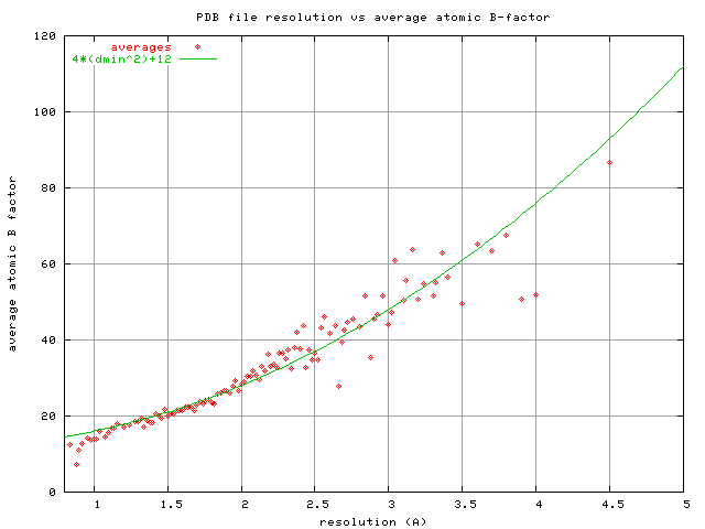
could have used the PDB-wide average atomic B factor reported for
structures with resolution "d", which roughly follows:
B = 4*d**2+12
https://bl831.als.lbl.gov/~jamesh/pickup/reso_vs_avgB.png
The reason I didn't use this formula for the movie is because I didn't
figure it out until about 10 years later. These two curves cross at
1.5A, but diverge significantly at poor resolution. So, which one is
right? It depends on how well you can measure really really faint
spots, and we've been getting better at that in recent decades.
So, what I'm trying to say here is that just because your data has CC1/2
or FSC dropping off to insignificance at 1.8 A doesn't mean you are
going to see holes in Tyr side chains. However, if you measure your
weak, high-res data really well (high multiplicity), you might be able
to sharpen your way to a much clearer map.
-James Holton
MAD Scientist
On 2/27/2020 11:01 AM, Nave, Colin (DLSLtd,RAL,LSCI) wrote:
James

All you say seems sensible to me but there is the possibility of
confusion regarding the use of the word threshold. I fully agree that
a half bit information threshold is inappropriate if it is taken to
mean that the data should be truncated at that resolution. The ever
more sophisticated refinement programs are becoming adept at handling
the noisy data.

The half bit information threshold I was discussing refers to a
nominal resolution. This is not just for trivial reporting purposes.
The half bit threshold is being used to compare imaging methods and
perhaps demonstrate that significant information is present with a
dose below any radiation damage threshold (that word again). The
justification for doing this appears to come from the fact it has been
adopted for protein structure determination by single particle
electron microscopy. However, low contrast features might not be
visible at this nominal resolution.

The analogy with protein crystallography might be to collect data
below an absorption edge to give a nominal resolution of 2 angstrom.
Then do it again well above the absorption edge. The second one gives
much greater Bijvoet differences despite the fact that the nominal
resolution is the same. I doubt whether anyone doing this would be
misled by this as they would examine the statistics for the Bijvoet
differences instead. However, it does indicate the relationship
between contrast and resolution.

The question, if referring to an information threshold for nominal
resolution, could be “Is there significant information in the data at
the required contrast and resolution?”. Then “Can one obtain this
information at a dose below any radiation damage limit”

Keep posting!

Regards

Colin

*From:*James Holton <[email protected]>
*Sent:* 27 February 2020 01:14
*To:* [email protected]
*Cc:* Nave, Colin (DLSLtd,RAL,LSCI) <[email protected]>
*Subject:* Re: [ccp4bb] [3dem] Which resolution?

In my opinion the threshold should be zero bits.  Yes, this is where
CC1/2 = 0 (or FSC = 0).  If there is correlation then there is
information, and why throw out information if there is information to
be had?  Yes, this information comes with noise attached, but that is
why we have weights.

It is also important to remember that zero intensity is still useful
information.  Systematic absences are an excellent example.  They have
no intensity at all, but they speak volumes about the structure.  In a
similar way, high-angle zero-intensity observations also tell us
something.  Ever tried unrestrained B factor refinement at poor
resolution?  It is hard to do nowadays because of all the safety
catches in modern software, but you can get great R factors this way.
A telltale sign of this kind of "over fitting" is remarkably large
Fcalc values beyond the resolution cutoff.  These don't contribute to
the R factor, however, because Fobs is missing for these hkls. So,
including zero-intensity data suppresses at least some types of
over-fitting.

The thing I like most about the zero-information resolution cutoff is
that it forces us to address the real problem: what do you mean by
"resolution" ?  Not long ago, claiming your resolution was 3.0 A meant
that after discarding all spots with individual I/sigI < 3 you still
have 80% completeness in the 3.0 A bin.  Now we are saying we have a
3.0 A data set when we can prove statistically that a few
non-background counts fell into the sum of all spot areas at 3.0 A.
These are not the same thing.

Don't get me wrong, including the weak high-resolution information
makes the model better, and indeed I am even advocating including all
the noisy zeroes.  However, weak data at 3.0 A is never going to be as
good as having strong data at 3.0 A.  So, how do we decide?  I
personally think that the resolution assigned to the PDB deposition
should remain the classical I/sigI > 3 at 80% rule.  This is really
the only way to have meaningful comparison of resolution between very
old and very new structures.  One should, of course, deposit all the
data, but don't claim that cut-off as your "resolution".  That is just
plain unfair to those who came before.

Oh yeah, and I also have a session on "interpreting low-resolution
maps" at the GRC this year.
https://www.grc.org/diffraction-methods-in-structural-biology-conference/2020/

So, please, let the discussion continue!

-James Holton
MAD Scientist

On 2/22/2020 11:06 AM, Nave, Colin (DLSLtd,RAL,LSCI) wrote:

     Alexis

     This is a very useful summary.

     You say you were not convinced by Marin's derivation in 2005. Are
     you convinced now and, if not, why?

     My interest in this is that the FSC with half bit thresholds have
     the danger of being adopted elsewhere because they are becoming
     standard for protein structure determination (by EM or MX). If it
     is used for these mature techniques it must be right!

     It is the adoption of the ½ bit threshold I worry about. I gave a
     rather weak example for MX which consisted of partial occupancy of
     side chains, substrates etc. For x-ray imaging a wide range of
     contrasts can occur and, if you want to see features with only a
     small contrast above the surroundings then I think the half bit
     threshold would be inappropriate.

     It would be good to see a clear message from the MX and EM
     communities as to why an information content threshold of ½ a bit
     is generally appropriate for these techniques and an
     acknowledgement that this threshold is technique/problem dependent.

     We might then progress from the bronze age to the iron age.

     Regards

     Colin

     *From:*CCP4 bulletin board <[email protected]>
     <mailto:[email protected]> *On Behalf Of *Alexis Rohou
     *Sent:* 21 February 2020 16:35
     *To:* [email protected] <mailto:[email protected]>
     *Subject:* Re: [ccp4bb] [3dem] Which resolution?

     Hi all,

     For those bewildered by Marin's insistence that everyone's been
     messing up their stats since the bronze age, I'd like to offer
     what my understanding of the situation. More details in this
     thread from a few years ago on the exact same topic:

     https://mail.ncmir.ucsd.edu/pipermail/3dem/2015-August/003939.html

     https://mail.ncmir.ucsd.edu/pipermail/3dem/2015-August/003944.html

     Notwithstanding notational problems (e.g. strict equations as
     opposed to approximation symbols, or omission of symbols to denote
     estimation), I believe Frank & Al-Ali and "descendent" papers
     (e.g. appendix of Rosenthal & Henderson 2003) are fine. The cross
     terms that Marin is agitated about indeed do in fact have an
     expectation value of 0.0 (in the ensemble; if the experiment were
     performed an infinite number of times with different realizations
     of noise). I don't believe Pawel or Jose Maria or any of the other
     authors really believe that the cross-terms are orthogonal.

     When N (the number of independent Fouier voxels in a shell) is
     large enough, mean(Signal x Noise) ~ 0.0 is only an approximation,
     but a pretty good one, even for a single FSC experiment. This is
     why, in my book, derivations that depend on Frank & Al-Ali are OK,
     under the strict assumption that N is large. Numerically, this
     becomes apparent when Marin's half-bit criterion is plotted -
     asymptotically it has the same behavior as a constant threshold.

     So, is Marin wrong to worry about this? No, I don't think so.
     There are indeed cases where the assumption of large N is broken.
     And under those circumstances, any fixed threshold (0.143, 0.5,
     whatever) is dangerous. This is illustrated in figures of van Heel
     & Schatz (2005). Small boxes, high-symmetry, small objects in
     large boxes, and a number of other conditions can make fixed
     thresholds dangerous.

     It would indeed be better to use a non-fixed threshold. So why am
     I not using the 1/2-bit criterion in my own work? While
     numerically it behaves well at most resolution ranges, I was not
     convinced by Marin's derivation in 2005. Philosophically though, I
     think he's right - we should aim for FSC thresholds that are more
     robust to the kinds of edge cases mentioned above. It would be the
     right thing to do.

     Hope this helps,

     Alexis

     On Sun, Feb 16, 2020 at 9:00 AM Penczek, Pawel A
     <[email protected] <mailto:[email protected]>>
     wrote:

         Marin,

         The statistics in 2010 review is fine. You may disagree with
         assumptions, but I can assure you the “statistics” (as you
         call it) is fine. Careful reading of the paper would reveal to
         you this much.

         Regards,

         Pawel


             On Feb 16, 2020, at 10:38 AM, Marin van Heel
             <[email protected]
             <mailto:[email protected]>> wrote:


             ***** EXTERNAL EMAIL *****

             Dear Pawel and All others ....

             This 2010 review is - unfortunately - largely based on the
             flawed statistics I mentioned before, namely on the a
             priori assumption that the inner product of a signal
             vector and a noise vector are ZERO (an orthogonality
             assumption).  The (Frank & Al-Ali 1975) paper we have
             refuted on a number of occasions (for example in 2005, and
             most recently in our BioRxiv paper) but you still take
             that as the correct relation between SNR and FRC (and you
             never cite the criticism...).

             Sorry

             Marin

             On Thu, Feb 13, 2020 at 10:42 AM Penczek, Pawel A
             <[email protected]
             <mailto:[email protected]>> wrote:

                 Dear Teige,

                 I am wondering whether you are familiar with


                     Resolution measures in molecular electron microscopy.

                 Penczek PA. Methods Enzymol. 2010.


                       Citation

                 Methods Enzymol. 2010;482:73-100. doi:
                 10.1016/S0076-6879(10)82003-8.

                 You will find there answers to all questions you asked
                 and much more.

                 Regards,

                 Pawel Penczek

                 Regards,

                 Pawel

                 _______________________________________________
                 3dem mailing list
                 [email protected] <mailto:[email protected]>
                 https://mail.ncmir.ucsd.edu/mailman/listinfo/3dem

<https://urldefense.proofpoint.com/v2/url?u=https-3A__mail.ncmir.ucsd.edu_mailman_listinfo_3dem&d=DwMFaQ&c=bKRySV-ouEg_AT-w2QWsTdd9X__KYh9Eq2fdmQDVZgw&r=yEYHb4SF2vvMq3W-iluu41LlHcFadz4Ekzr3_bT4-qI&m=3-TZcohYbZGHCQ7azF9_fgEJmssbBksaI7ESb0VIk1Y&s=XHMq9Q6Zwa69NL8kzFbmaLmZA9M33U01tBE6iAtQ140&e=>

         _______________________________________________
         3dem mailing list
         [email protected] <mailto:[email protected]>
         https://mail.ncmir.ucsd.edu/mailman/listinfo/3dem

     ------------------------------------------------------------------------

     To unsubscribe from the CCP4BB list, click the following link:
     https://www.jiscmail.ac.uk/cgi-bin/webadmin?SUBED1=CCP4BB&A=1

     --

     This e-mail and any attachments may contain confidential,
     copyright and or privileged material, and are for the use of the
     intended addressee only. If you are not the intended addressee or
     an authorised recipient of the addressee please notify us of
     receipt by returning the e-mail and do not use, copy, retain,
     distribute or disclose the information in or attached to the e-mail.
     Any opinions expressed within this e-mail are those of the
     individual and not necessarily of Diamond Light Source Ltd.
     Diamond Light Source Ltd. cannot guarantee that this e-mail or any
     attachments are free from viruses and we cannot accept liability
     for any damage which you may sustain as a result of software
     viruses which may be transmitted in or with the message.
     Diamond Light Source Limited (company no. 4375679). Registered in
     England and Wales with its registered office at Diamond House,
     Harwell Science and Innovation Campus, Didcot, Oxfordshire, OX11
     0DE, United Kingdom

     ------------------------------------------------------------------------

     To unsubscribe from the CCP4BB list, click the following link:
     https://www.jiscmail.ac.uk/cgi-bin/webadmin?SUBED1=CCP4BB&A=1

--

This e-mail and any attachments may contain confidential, copyright
and or privileged material, and are for the use of the intended
addressee only. If you are not the intended addressee or an authorised
recipient of the addressee please notify us of receipt by returning
the e-mail and do not use, copy, retain, distribute or disclose the
information in or attached to the e-mail.
Any opinions expressed within this e-mail are those of the individual
and not necessarily of Diamond Light Source Ltd.
Diamond Light Source Ltd. cannot guarantee that this e-mail or any
attachments are free from viruses and we cannot accept liability for
any damage which you may sustain as a result of software viruses which
may be transmitted in or with the message.
Diamond Light Source Limited (company no. 4375679). Registered in
England and Wales with its registered office at Diamond House, Harwell
Science and Innovation Campus, Didcot, Oxfordshire, OX11 0DE, United
Kingdom
########################################################################

To unsubscribe from the CCP4BB list, click the following link:
https://www.jiscmail.ac.uk/cgi-bin/webadmin?SUBED1=CCP4BB&A=1